Hypothesis testing: confident conclusions
Hypothesis testing determines if data supports a specific hypothesis. TableTorch supports the following tests:
- Analysis of variance (ANOVA) F-test compares variances across groups to find significant differences.
- Student’s T-test evaluates if the means of two groups significantly differ, aiding in decision-making based on statistical evidence.
In this article, we’ll explore possible applications of hypothesis testing and perform analysis of UI experiment data using TableTorch’s hypothesis testing feature.
- Key features:
- Examples of hypothesis testing application
- Calculating statistical tests for UI experiment data: a quick guide
Key features:
- Multiple groups: Choose data columns for analysis, with one serving as a control group.
- Statistical tests:
- One-way ANOVA F-test: Compares variances across multiple groups to determine if any substantial differences exist.
- One-sample T-test: Tests if the sample mean differs from a known population mean (μ0). Ideal for hypothesis testing against a specific benchmark.
- Dependent (paired) T-test: Compares means from two related groups. Perfect for before-and-after studies.
- Independent two-sample T-test: Assesses if the means of two independent groups are significantly different. Useful for comparing two distinct groups.
- μ0 (population mean) setting: Easily set μ0 to either the mean of selected groups or the control group mean.
- UI is the spreadsheet itself: Computation results are presented in a new sheet containing:
- test statistics and p-values for selected tests.
- common measures (average, median, 25th and 75th percentiles, standard deviation) displayed in table and a chart.
Examples of hypothesis testing application
- Marketing Effectiveness: Determine the impact of marketing campaigns by comparing conversion rates.
- Process Changes: Assess the effects of changes in processes on productivity.
- Customer Satisfaction: Evaluate satisfaction levels before and after service modifications.
- Quality Control: Identify significant differences in product defects across different production batches.
- Data-Driven Decisions, A/B testing: Empower businesses to validate assumptions and improve operational efficiency.
- Academic Research: Test hypotheses and validate theories in social sciences, natural sciences, and humanities.
- Educational Assessments: Compare student performance before and after implementing new teaching methods or curricula.
Calculating statistical tests for UI experiment data: a quick guide
To better understand the Hypothesis testing function of TableTorch, let’s explore a worked-out experiment example.
Experiment overview
A large enterprise aims to simplify their ERP system’s UI to help employees find inventory faster. Before a full rollout, they conducted an experiment with three employee groups:
- Control: No UI changes; serves as the baseline.
- Distraction: Minor visual changes to test if any effect is due to novelty.
- New design: Significant UI changes to reduce search iterations.
The experiment will determine if the new design improves efficiency and if further investment is justified.
Experiment method
The experimenter should follow these steps:
- Recruit 150 employees for the experiment, ensuring each consents to participate. Randomly assign them to three equal groups.
- Observe and record the average search time for inventory using the current UI for one day. Extract data from the ERP system.
- Perform an ANOVA F-test to check if the variance in search times between groups is due to random variation.
- If the p-value is greater than 0.05, assume the variance is random.
- If not, reassign participants and recalculate until the p-value is high.
- Implement the UI changes and record the average search time as done in step 2.
- Conduct an independent Student’s t-test between the Control, Distraction, and New design groups.
- Check if the New design mean is at least 5% lower than the Control mean.
- If the New design change in time is downward and statistically significant and that’s not the case for the Distraction group, deem the hypothesis confirmed.
- Otherwise, stop the experiment and accept the null hypothesis.
- Perform a dependent Student’s t-test for the New design group before and after the change.
- Check if the mean search time is at least 5% lower.
- If the p-value is above 0.05, cancel the experiment and accept the null hypothesis.
- If successful, present the analysis to management, showing data supports increased productivity.
Before discussing the dataset and statistical tests, please ensure you have installed the TableTorch add-on. See the instructions below to find out how to do that.
Start TableTorch
- Install TableTorch to Google Sheets via Google Workspace Marketplace. More details on initial setup.
- Click on the TableTorch icon
on right-side panel of Google Sheets.
Steps 1-3: Before change
Step 1: recruiting 150 employees for the experiment
150 employees were recruited and each gave a written consent to take part in the experiment.
Step 2: collecting a sheet with data before design change
This sheet shows the average time (in seconds) it took employees to find an inventory item in the first day of experiment, before any UI changes. Each column represents a different group in the experiment.
| A | B | C |
|---|---|---|
| Control | Distraction | New Design |
| 9.7 | 13.4 | 9.7 |
| 10.0 | 9.3 | 13.9 |
| 11.1 | 11.5 | 10.9 |
| 10.7 | 13.3 | 12.4 |
| 14.1 | 12.3 | 11.5 |
| 10.8 | 11.0 | 13.8 |
| 10.8 | 14.1 | 11.6 |
| 12.3 | 12.0 | 12.5 |
| 9.5 | 11.7 | 13.6 |
| 12.4 | 13.2 | 12.5 |
| 14.4 | 15.7 | 12.7 |
| 13.0 | 11.0 | 12.3 |
| 13.3 | 12.5 | 13.6 |
| 12.8 | 12.7 | 11.4 |
| 10.8 | 14.1 | 14.6 |
| 13.9 | 11.1 | 12.1 |
| 10.9 | 12.1 | 8.9 |
| 9.1 | 11.1 | 12.5 |
| 12.1 | 11.9 | 11.8 |
| 13.4 | 11.9 | 12.4 |
| 12.4 | 12.2 | 15.0 |
| 9.3 | 12.1 | 12.0 |
| 11.0 | 11.7 | 11.9 |
| 12.5 | 12.0 | 12.4 |
| 12.9 | 11.7 | 8.3 |
| 12.4 | 10.3 | 11.5 |
| 12.3 | 13.7 | 13.0 |
| 12.2 | 11.5 | 12.5 |
| 13.4 | 10.5 | 10.4 |
| 14.9 | 10.4 | 13.9 |
| 11.3 | 12.1 | 11.6 |
| 10.4 | 11.9 | 7.7 |
| 11.4 | 13.4 | 9.8 |
| 12.4 | 12.7 | 15.5 |
| 14.5 | 14.7 | 11.2 |
| 10.4 | 13.3 | 13.2 |
| 11.5 | 9.4 | 11.3 |
| 10.3 | 13.4 | 10.4 |
| 12.5 | 11.2 | 13.1 |
| 10.8 | 10.6 | 13.8 |
| 10.3 | 9.6 | 10.4 |
| 11.5 | 10.8 | 13.5 |
| 12.6 | 14.3 | 13.5 |
| 13.1 | 9.5 | 13.7 |
| 14.2 | 12.4 | 13.2 |
| 9.3 | 10.3 | 11.8 |
| 11.1 | 13.7 | 13.1 |
| 10.8 | 11.8 | 12.5 |
| 12.7 | 14.1 | 13.7 |
| 12.0 | 12.6 | 12.5 |
Step 3: Attribution of variance to random chance
The average time (in seconds) among all the groups is 12.04 but there’s a slight difference between the groups:
- Control: 11.8 minutes
- Distraction: 12.1 minutes
- New Design: 12.2 minutes
To ensure fair group distribution and avoid bias, we perform an ANOVA F-test, one-sample Student’s t-test and examine associated with respective scores p-values. If a p-value is below 0.05, the differences are likely significant and not due to random chance.
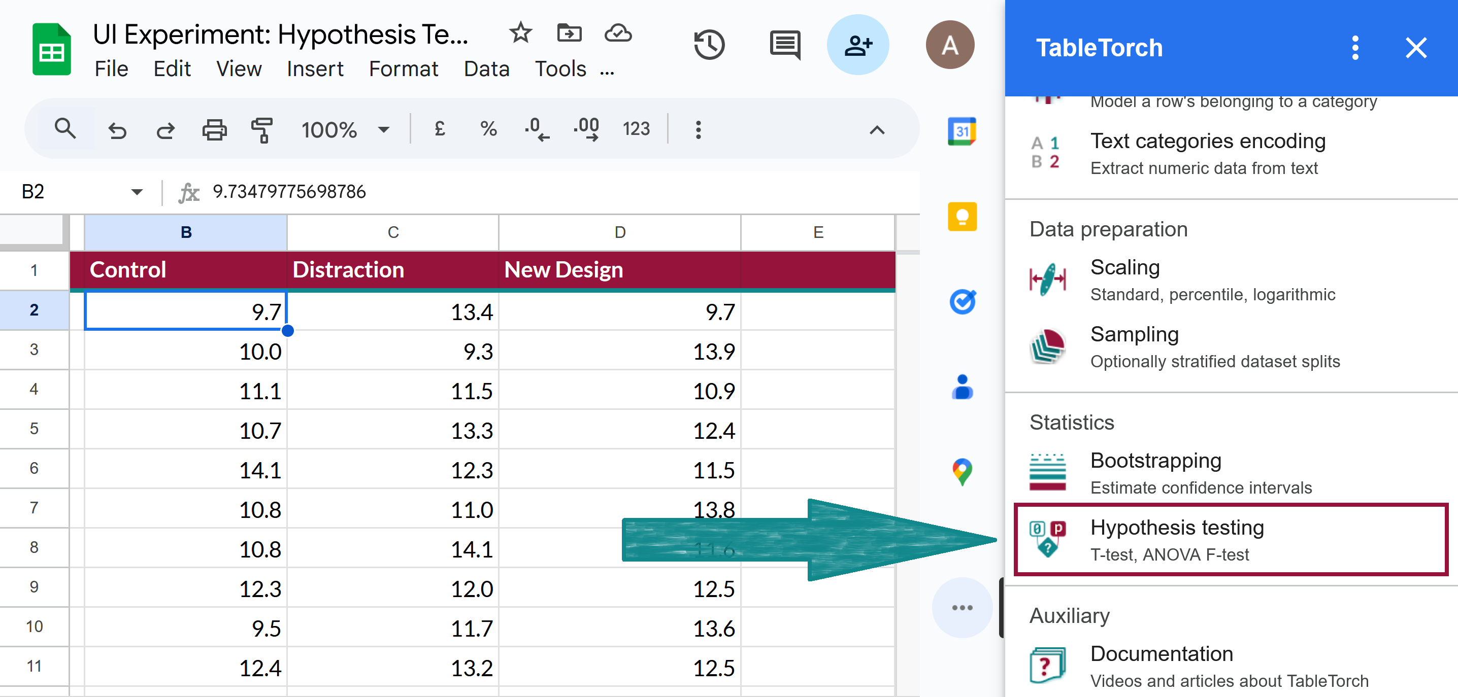
➡️ Select the first cell of the data table on the sheet, open TableTorch, and click the Hypothesis testing item on its main menu.
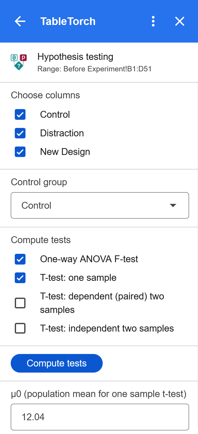
➡️ Check One-way ANOVA F-test and T-test: one sample, enter 12.04 for μ0 and click Compute tests.
NOTE: Control group doesn’t matter in this computation because neither of two sample T-test options were selected.
➡️ Examine the inserted sheet with results:
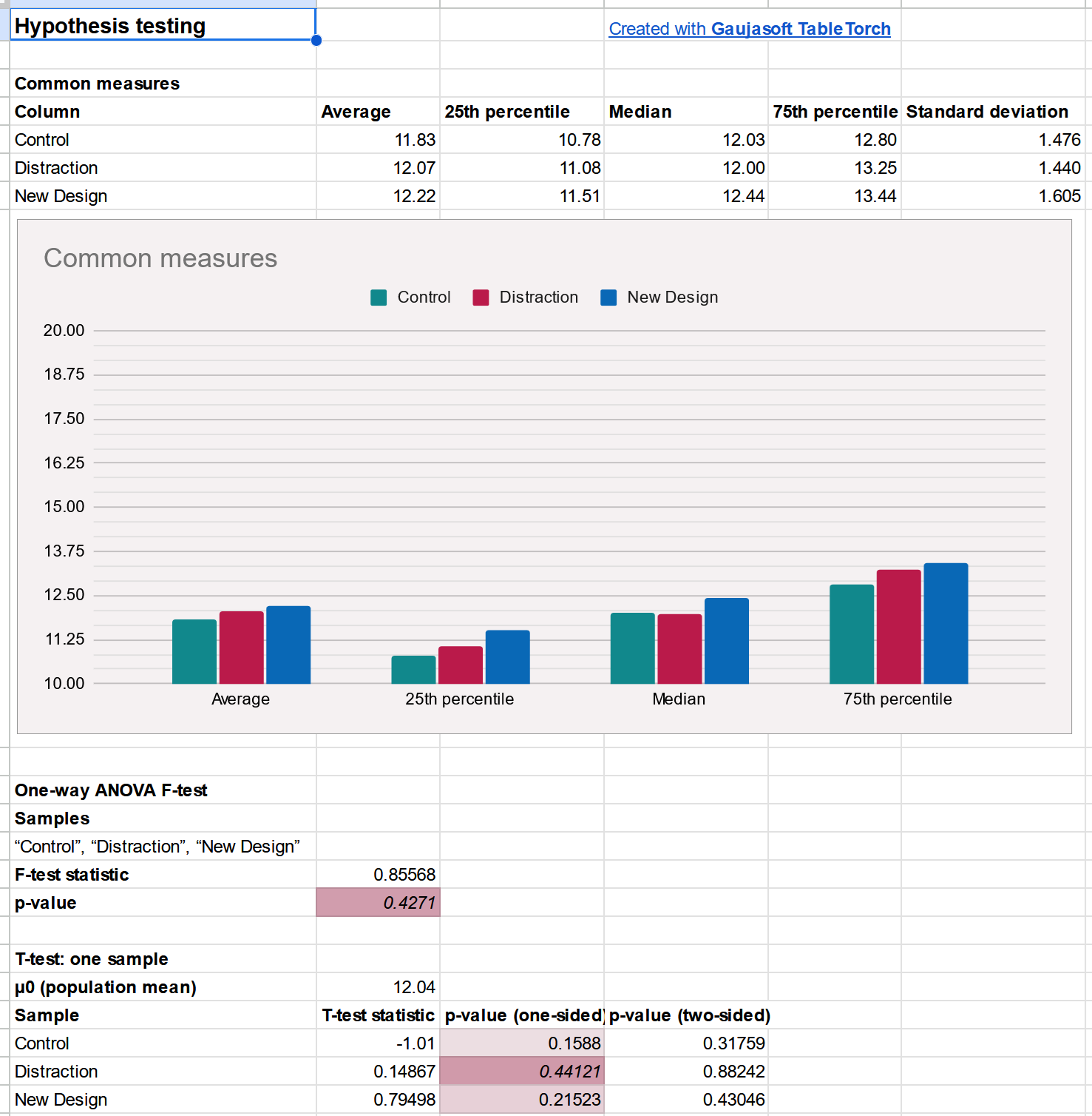
Here’s what we see on the sheet:
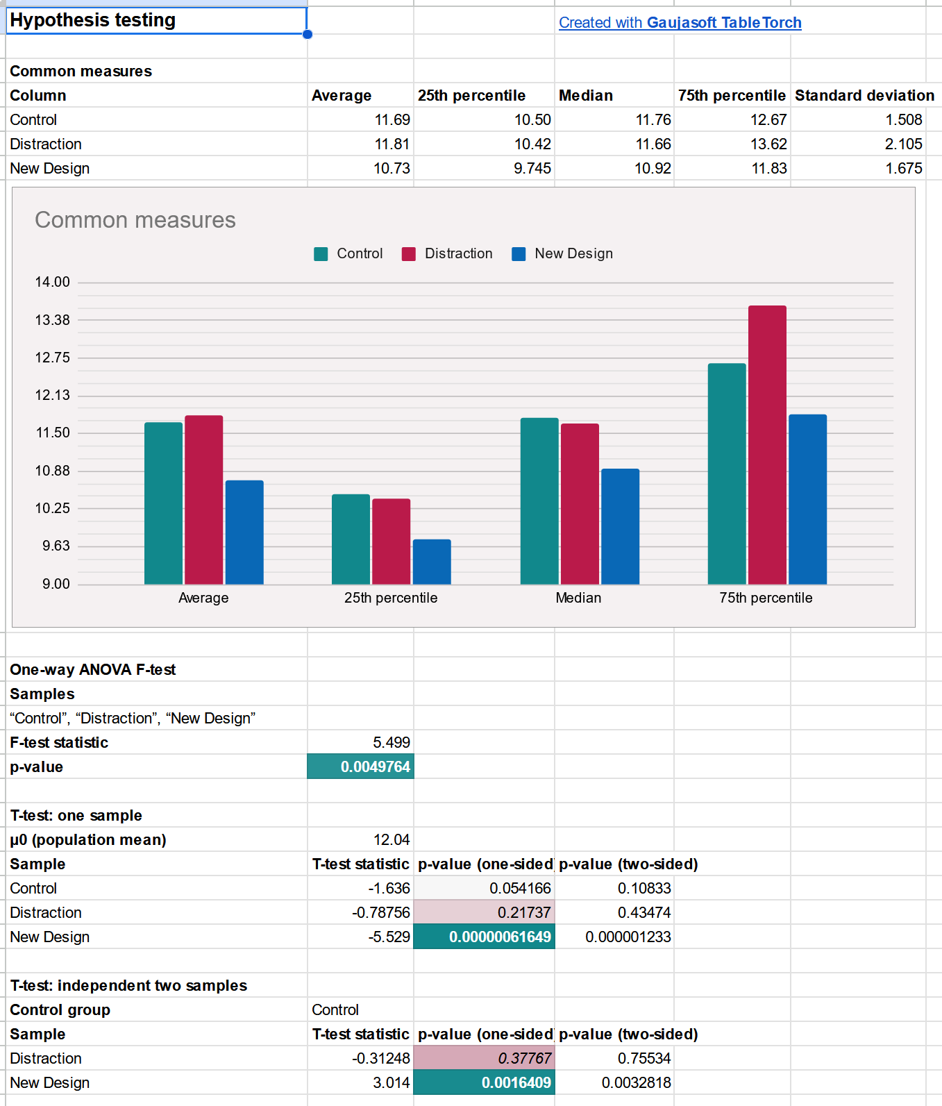
- Common measures, displayed both as a table and a corresponding chart, show negligible difference across the groups.
- F-test’s associated p-value at 0.43 clearly signals that the differences in variance between the groups are not statistically significant.
- One sample t-tests for all the groups show associated two-sided p-values much larger than 0.05, confirming that the differences in means across the groups are also not statistically significant.
Fortunately, both the ANOVA F-test and the one sample t-tests didn’t show any statistically significant differences between the groups. This helps us make sure that we can continue with the experiment as planned and shall not be afraid of uneven or biased selection of participants into the groups.
Steps 4-6: After change
Step 4: implementing change and collecting new data
Once the design changes were applied to the Distraction and New Design groups, new data was collected. Three new sheets were added to the spreadsheet:
- After Change: three columns containing the groups’ data in the same way as the sheet from step 2.
- Before/After: Distraction: sheet with two columns; the first represents the Distraction group’s participants before UI changes and the second represents the same participants after UI changes were introduced.
- Before/After: New Design: sheet with two columns about the New Design group of experiment’s participants.
Step 4.1: After Change Sheet
This sheets was collected in the same way as the initial dataset but after the design changes were introduced.
| A | B | C |
|---|---|---|
| Control | Distraction | New Design |
| 10.3 | 13.0 | 8.1 |
| 9.2 | 7.1 | 13.2 |
| 11.1 | 7.7 | 9.2 |
| 10.6 | 14.1 | 9.6 |
| 12.9 | 11.7 | 10.6 |
| 10.7 | 10.4 | 12.1 |
| 10.4 | 12.4 | 9.7 |
| 11.8 | 11.4 | 10.3 |
| 10.2 | 11.0 | 11.8 |
| 11.7 | 13.7 | 11.8 |
| 15.0 | 15.8 | 11.3 |
| 12.6 | 10.0 | 10.9 |
| 12.4 | 14.5 | 12.3 |
| 12.3 | 11.3 | 9.7 |
| 11.4 | 15.1 | 12.7 |
| 13.8 | 12.0 | 9.9 |
| 10.5 | 13.5 | 8.1 |
| 9.7 | 9.2 | 10.4 |
| 11.8 | 12.5 | 11.4 |
| 13.5 | 12.6 | 10.7 |
| 12.4 | 13.7 | 13.8 |
| 9.3 | 11.7 | 10.9 |
| 10.4 | 10.7 | 10.7 |
| 13.0 | 12.1 | 10.5 |
| 13.4 | 12.8 | 6.8 |
| 11.8 | 10.9 | 10.0 |
| 13.1 | 15.1 | 10.9 |
| 12.2 | 11.2 | 10.8 |
| 13.9 | 9.0 | 8.9 |
| 15.4 | 9.8 | 12.2 |
| 10.1 | 11.4 | 11.0 |
| 10.8 | 10.6 | 6.4 |
| 12.6 | 14.9 | 8.4 |
| 12.6 | 14.0 | 14.5 |
| 13.3 | 13.0 | 9.1 |
| 10.2 | 11.8 | 11.5 |
| 10.9 | 7.7 | 10.0 |
| 9.7 | 13.8 | 8.5 |
| 12.1 | 11.0 | 12.6 |
| 10.9 | 10.2 | 12.1 |
| 10.2 | 8.6 | 8.5 |
| 11.1 | 9.3 | 11.8 |
| 11.9 | 14.9 | 12.3 |
| 12.8 | 11.6 | 11.6 |
| 14.2 | 12.5 | 11.3 |
| 8.9 | 10.0 | 10.9 |
| 10.6 | 14.3 | 11.7 |
| 10.6 | 11.4 | 11.8 |
| 12.7 | 14.2 | 11.9 |
| 11.4 | 9.7 | 11.6 |
Step 4.2: Before/After: Distraction Sheet
In this sheet, each row represents average time (in seconds) it took a particular participant of the Distraction group to find an inventory item before and after the UI changes were introduced.
| A | B |
|---|---|
| Distraction: Before | Distraction: After |
| 13.4 | 13.0 |
| 9.3 | 7.1 |
| 11.5 | 7.7 |
| 13.3 | 14.1 |
| 12.3 | 11.7 |
| 11.0 | 10.4 |
| 14.1 | 12.4 |
| 12.0 | 11.4 |
| 11.7 | 11.0 |
| 13.2 | 13.7 |
| 15.7 | 15.8 |
| 11.0 | 10.0 |
| 12.5 | 14.5 |
| 12.7 | 11.3 |
| 14.1 | 15.1 |
| 11.1 | 12.0 |
| 12.1 | 13.5 |
| 11.1 | 9.2 |
| 11.9 | 12.5 |
| 11.9 | 12.6 |
| 12.2 | 13.7 |
| 12.1 | 11.7 |
| 11.7 | 10.7 |
| 12.0 | 12.1 |
| 11.7 | 12.8 |
| 10.3 | 10.9 |
| 13.7 | 15.1 |
| 11.5 | 11.2 |
| 10.5 | 9.0 |
| 10.4 | 9.8 |
| 12.1 | 11.4 |
| 11.9 | 10.6 |
| 13.4 | 14.9 |
| 12.7 | 14.0 |
| 14.7 | 13.0 |
| 13.3 | 11.8 |
| 9.4 | 7.7 |
| 13.4 | 13.8 |
| 11.2 | 11.0 |
| 10.6 | 10.2 |
| 9.6 | 8.6 |
| 10.8 | 9.3 |
| 14.3 | 14.9 |
| 9.5 | 11.6 |
| 12.4 | 12.5 |
| 10.3 | 10.0 |
| 13.7 | 14.3 |
| 11.8 | 11.4 |
| 14.1 | 14.2 |
| 12.6 | 9.7 |
Step 4.3: Before/After: New Design Sheet
Each row represents mean timing (in seconds) for a particular participant of the New Design group before and after the redesign.
| A | B |
|---|---|
| New Design: Before | New Design: After |
| 9.7 | 8.1 |
| 13.9 | 13.2 |
| 10.9 | 9.2 |
| 12.4 | 9.6 |
| 11.5 | 10.6 |
| 13.8 | 12.1 |
| 11.6 | 9.7 |
| 12.5 | 10.3 |
| 13.6 | 11.8 |
| 12.5 | 11.8 |
| 12.7 | 11.3 |
| 12.3 | 10.9 |
| 13.6 | 12.3 |
| 11.4 | 9.7 |
| 14.6 | 12.7 |
| 12.1 | 9.9 |
| 8.9 | 8.1 |
| 12.5 | 10.4 |
| 11.8 | 11.4 |
| 12.4 | 10.7 |
| 15.0 | 13.8 |
| 12.0 | 10.9 |
| 11.9 | 10.7 |
| 12.4 | 10.5 |
| 8.3 | 6.8 |
| 11.5 | 10.0 |
| 13.0 | 10.9 |
| 12.5 | 10.8 |
| 10.4 | 8.9 |
| 13.9 | 12.2 |
| 11.6 | 11.0 |
| 7.7 | 6.4 |
| 9.8 | 8.4 |
| 15.5 | 14.5 |
| 11.2 | 9.1 |
| 13.2 | 11.5 |
| 11.3 | 10.0 |
| 10.4 | 8.5 |
| 13.1 | 12.6 |
| 13.8 | 12.1 |
| 10.4 | 8.5 |
| 13.5 | 11.8 |
| 13.5 | 12.3 |
| 13.7 | 11.6 |
| 13.2 | 11.3 |
| 11.8 | 10.9 |
| 13.1 | 11.7 |
| 12.5 | 11.8 |
| 13.7 | 11.9 |
| 12.5 | 11.6 |
Step 5: independent Student’s t-test
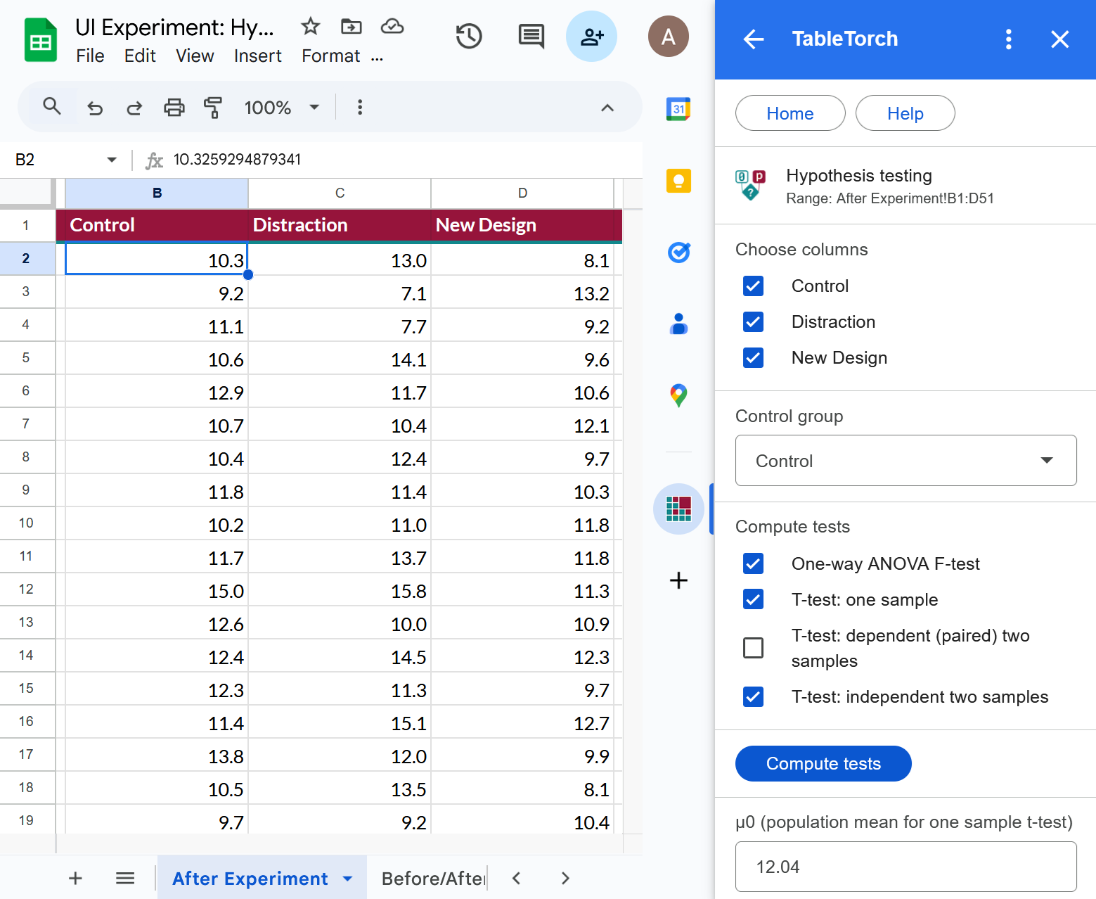
- ➡️ Open the After Change sheet, select the first cell of the data table, open TableTorch and click the Hypothesis testing menu item.
- Select Control column in the Control group dropdown (it will probably be there by default).
- Select tests to compute:
- One-way ANOVA F-test
- T-test: one sample
- T-test: independent two samples
- Enter 12.04 for μ0 (population mean).
- Click Compute tests.
Configuration:
Resulting sheet:
Summary:
- The common measures chart clearly shows that the New Design group’s participants found the necessary inventory items slightly faster (average time is 0.9 seconds or about 8% lower than that of the Control group), whether average, median, 25th or 75th percentile is compared.
- F-test’s associated p-value at 0.005 signals that the difference in variance between the groups is highly unlikely due to random chance only.
- One sample t-tests:
- show associated two-sided p-values higher than 0.05 for both the Control and Distraction groups, meaning that those groups’ variation from population’s average collected in the initial data is not statistically significant.
- display one-sided p-value for the New Design group much lower than 0.05, confirming that the difference is statistically significant.
- Independent two samples t-tests:
- difference in mean for Distraction group is not statistically significant.
- change in the required time for New Design group is statistically significant.
These results alone are enough to present them to the management and defend the case to expand the new design’s coverage of inventory and enable it for all the ERP users eventually.
However, for the sake of this article’s completeness, let’s calculate the dependent two sample t-tests as well.
Step 6: dependent (paired) Student’s t-tests
In the previous section, we used independent Student’s t-tests to compare the Distraction and New Design groups with the Control group. In this context, individual rows are less significant, as each cell represents the timings of different participants.
However, using the data from Before/After: Distraction and Before/After: New Design sheets, where each row represents a single participant and columns show timings before and after the UI changes respectively, it is possible to perform probably more detailed, paired (dependent) t-tests.
Step 6.1: paired t-test for the Distraction group
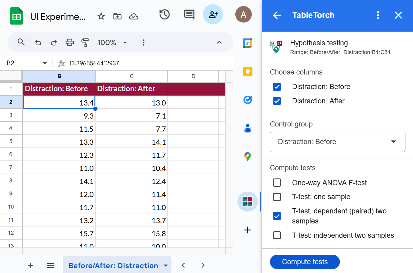
- ➡️ Open the Before/After: Distraction sheet, select any cell of the data table, open TableTorch and click the Hypothesis testing menu item.
- Select Distraction: Before column in the Control group dropdown (it is most likely the default value).
- Check only T-test: dependent (paired) two samples test to compute.
- Click Compute tests.
Configuration:
Resulting sheet:
Summary:
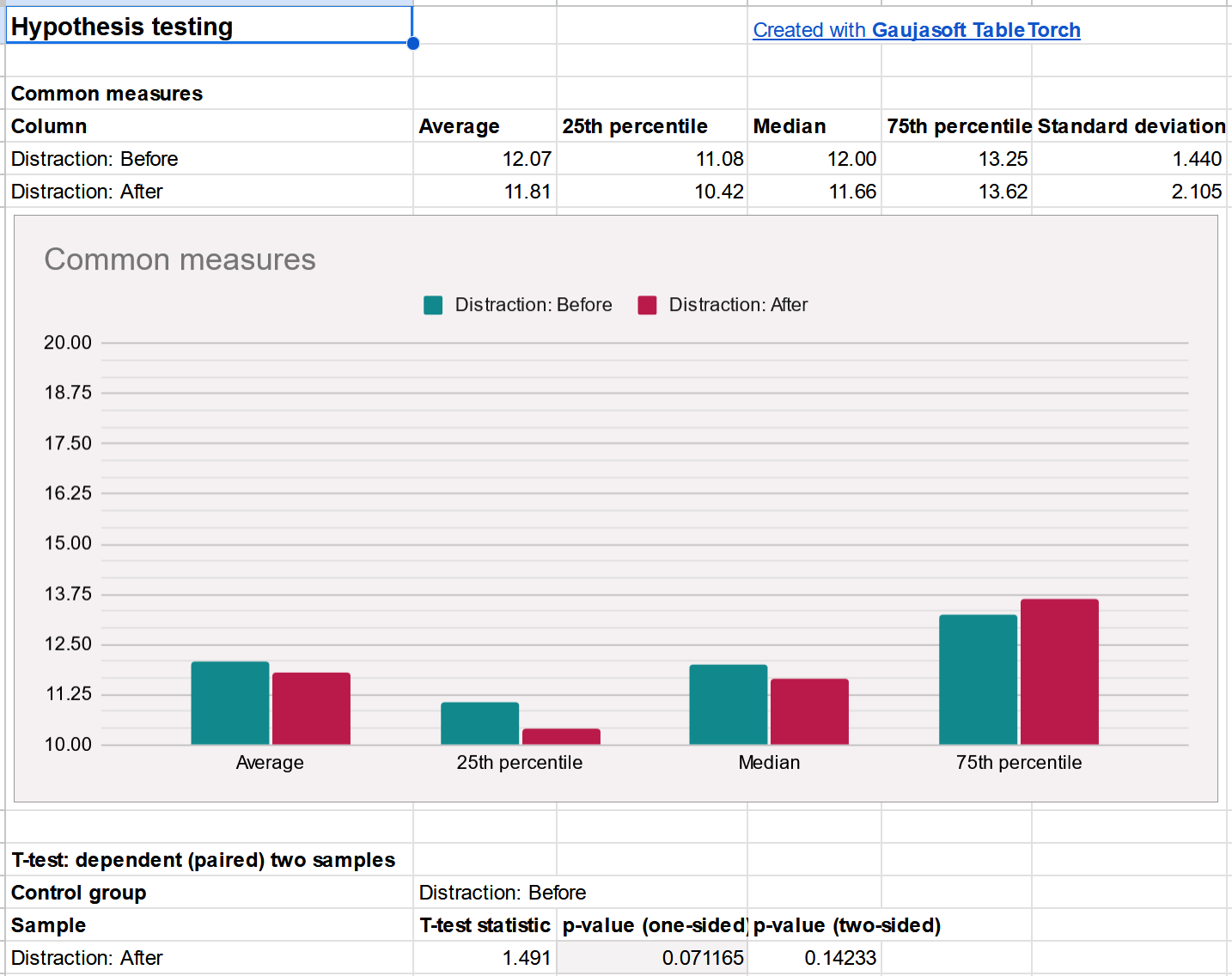
- The common measures displayed on the chart show that the timings are slightly lower on average, as well as for the 25th percentile and even the median participant. However, they are greater for the 75th percentile, suggesting that the difference might be explained by the expanded variance due to the novelty of the design.
- Associated two-sided p-value at 0.14 indicates that the difference is not statistically significant.
Step 6.2: paired t-test for the New Design group
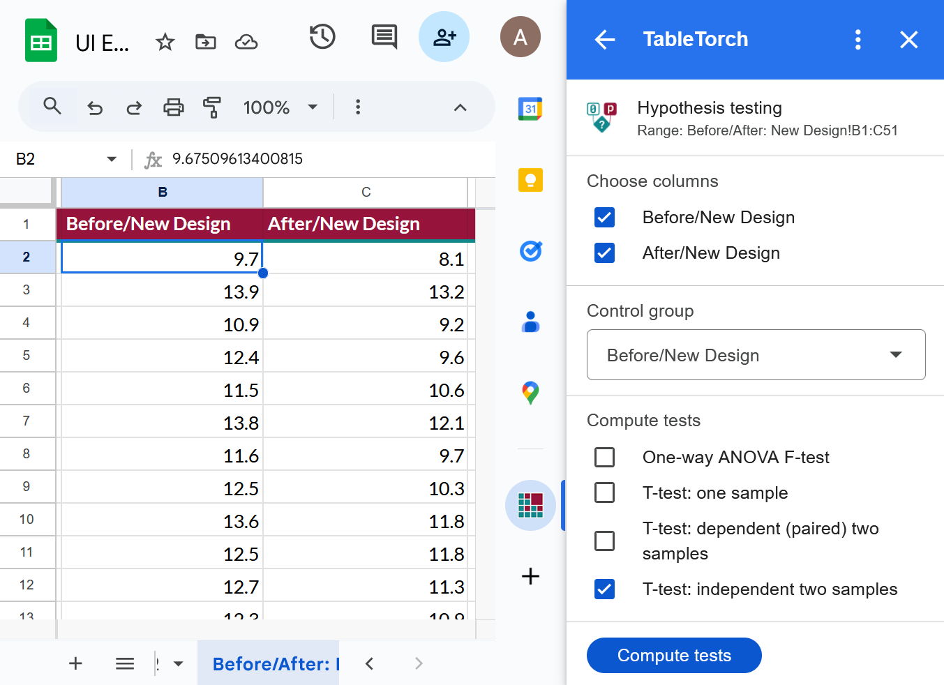
- ➡️ Open the Before/After: New Design sheet, select any cell of the data table, open TableTorch and click the Hypothesis testing menu item.
- Select New Design: Before column in the Control group dropdown (it is most likely the default value).
- Check only T-test: dependent (paired) two samples test to compute.
- Click Compute tests.
Configuration:
Resulting sheet:
Summary:
- All the common measures (mean, median, 25th and 75th percentiles) show lower timings after the redesign.
- Paired t-test’s associated one-sided p-value is much mower than 0.05, indicating that the change is statistically significant.
Step 7: drawing conclusions
For a simple experiment like this, just looking at the charts might be sufficient for the management to make an appropriate decision. However, TableTorch can quickly compute statistical tests such as ANOVA F-test and Student’s t-test thus helping presenter to improve their argument defending the case for a continuation of UI redesign effort, showing that the productivity improvement is tangible and statistically significant. Furthermore, the numbers are often more complex than they appear, and relying solely on averages and charts can sometimes mislead an observer.
Note regarding one-sided and two-sided p-values
TableTorch computes both the one-sided and two-sided associated p-values for ANOVA F-test and Student’s t-tests. It is important that you choose which one to use to determine the statistical significance beforehand.
- One-Sided p-value: Tests the hypothesis that there is a significant effect in one specific direction (either an increase or decrease). Use it when the direction of the effect is known.
- Two-Sided p-value: Tests the hypothesis that there is a significant effect in either direction (both increase and decrease). It is used when there is no prior assumption about the direction of the effect.
Google, Google Sheets, Google Workspace and YouTube are trademarks of Google LLC. Gaujasoft TableTorch is not endorsed by or affiliated with Google in any way.
Let us know!
Thank you for using or considering to use TableTorch!
Does this page accurately and appropriately describe the function in question? Does it actually work as explained here or is there any problem? Do you have any suggestion on how we could improve?
Please let us know if you have any questions.
- E-mail: ___________
- Facebook page
- Twitter profile

